Beam Loss Monitor Query with pyeDSL
The goal of this blog entry is to demontrate the use of the pyeDSL to conventiently query BLM-related data from Post Mortem (PM) and NXCALS databases. In particular, we will show how to query for a given period of time around an interesting event in the LHC:
- LHC context information from PM
- BLM signals from PM for plotting and extraction of statistical features (min, max, etc.)
- BLM signals from NXCALS for extraction of statistical features (min, max, etc.)
The PM queries presented below are partially based on previous work of:
- M. Valette: https://gitlab.cern.ch/LHCData/PostMortemData
- M. Dziadosz, R. Schmidt, L. Grob: https://gitlab.cern.ch/UFO/PMdataAnalysis
We found useful a presentation on BLM logging: https://indico.cern.ch/event/20366/contributions/394830/attachments/307939/429949/BLM_6th_Radiation_Workshop_Christos.pdf
0. Import Necessary Packages
- Time is a class for time manipulation and conversion
- Timer is a class for measuring time of code execution
- QueryBuilder is a pyeDSL class for a construction of database queries
- PmDbRequest is a low-level class for executing PM queries
- MappingMetadata is a class for retrieving BLM table names for NXCALS query
- BlmAnalysis class provides some helper functions for BLM Analysis
In [2]:
import pandas as pd
from lhcsmapi.Time import Time
from lhcsmapi.Timer import Timer
from lhcsmapi.pyedsl.QueryBuilder import QueryBuilder
from lhcsmapi.pyedsl.FeatureBuilder import FeatureBuilder
from lhcsmapi.dbsignal.post_mortem.PmDbRequest import PmDbRequest
from lhcsmapi.metadata.MappingMetadata import MappingMetadata
import lhcsmapi.analysis.BlmAnalysis as BlmAnalysis
0.1. LHCSMAPI version
In [3]:
import lhcsmapi
lhcsmapi.__version__
Out[3]:
'1.3.157'1. User Input
We choose as a start date a beam dump in the LHC. In this case, PM stores a data event with information about LHC context and BLM signals. In order to find PM events, we look one second before and two seconds after the selected beam dump.
NXCALS database performs a continuous logging of BLM signals (with various running sums). Thus, NXCALS can be queried any time.
In [4]:
start_time_date = '2015-11-23 07:28:53+01:00'
t_start, t_end = Time.get_query_period_in_unix_time(start_time_date=start_time_date, duration_date=[(1, 's'), (2, 's')])
2. LHC Context
In this part we query LHC context information in order to support BLM analysis. To this end, we employ context_query provided by pyeDSL.
- The context_query() works only in a general-purpose query mode with metadata provided by with_query_parameters() method. Considering the general-purpose mode, the user has to provide system, className, and source.
For the source field one can use a wildcard ('*'). However, the query takes more time as compared to a one where the BLM source is specified. The list of available BLM source can be queried from PM as showed in the following.
In [5]:
with Timer():
    QueryBuilder().with_pm() \
        .with_duration(t_start=t_start, duration=[(2, 's')]) \
        .with_query_parameters(system='BLM', className='BLMLHC', source='*') \
        .context_query(contexts=["pmFillNum"]).df
Elapsed: 21.443 s.
In [6]:
with Timer():
    QueryBuilder().with_pm() \
        .with_duration(t_start=t_start, duration=[(2, 's')]) \
        .with_query_parameters(system='BLM', className='BLMLHC', source='HC.BLM.SR6.C') \
        .context_query(contexts=["pmFillNum"]).df
Elapsed: 1.403 s.
Therefore, for the remaining context queries we always provide the source.
In [7]:
QueryBuilder().with_pm() \
    .with_duration(t_start=t_start, duration=[(2, 's')]) \
    .with_query_parameters(system='LHC', className='CISX', source='CISX.CCR.LHC.A') \
    .context_query(contexts=["OVERALL_ENERGY", "OVERALL_INTENSITY_1", "OVERALL_INTENSITY_2"]).df
Out[7]:
| OVERALL_ENERGY | OVERALL_INTENSITY_1 | OVERALL_INTENSITY_2 | |
|---|---|---|---|
| 1448260133517488525 | 20915 | 16537 | 17110 |
In [8]:
QueryBuilder().with_pm() \
    .with_duration(t_start=t_start, duration=[(2, 's')]) \
    .with_query_parameters(system='LHC', className='CISX', source='CISX.CCR.LHC.GA') \
    .context_query(contexts=["BEAM_MODE"]).df
Out[8]:
| BEAM_MODE | |
|---|---|
| 1448260133517488525 | 11 |
In [9]:
QueryBuilder().with_pm() \
    .with_duration(t_start=t_start, duration=[(5, 's')]) \
    .with_query_parameters(system='LBDS', className='BSRA', source='LHC.BSRA.US45.B1') \
    .context_query(contexts=['aGXpocTotalIntensity', 'aGXpocTotalMaxIntensity']).df
Out[9]:
| aGXpocTotalIntensity | aGXpocTotalMaxIntensity | |
|---|---|---|
| 1448260134624467000 | 2.457193e+10 | 8.560893e+08 |
In [10]:
QueryBuilder().with_pm() \
    .with_duration(t_start=t_start, duration=[(5, 's')]) \
    .with_query_parameters(system='LBDS', className='BSRA', source='LHC.BSRA.US45.B2') \
    .context_query(contexts=['aGXpocTotalIntensity', 'aGXpocTotalMaxIntensity']).df
Out[10]:
| aGXpocTotalIntensity | aGXpocTotalMaxIntensity | |
|---|---|---|
| 1448260134624467000 | 4.608540e+09 | 1.917766e+08 |
We also developed a method for getting the LHC context shown above with a single method.
In [11]:
lhc_context_df = BlmAnalysis.get_lhc_context(start_time_date)
lhc_context_df
Out[11]:
| OVERALL_ENERGY | OVERALL_INTENSITY_1 | OVERALL_INTENSITY_2 | BEAM_MODE | timestamp_blm | aGXpocTotalIntensityB1 | aGXpocTotalMaxIntensityB1 | aGXpocTotalIntensityB2 | aGXpocTotalMaxIntensityB2 | timestamp_abort_gap | |
|---|---|---|---|---|---|---|---|---|---|---|
| 4647 | 25098.0 | 16537 | 17110 | STABLE | 1448260133517488525 | 2.457193e+10 | 8.560893e+08 | 4.608540e+09 | 1.917766e+08 | 1448260134624467000 |
3. Query Single BLM
Once the LHC context is obtained, we move on to the query of BML signals with PM and NXCALS.
3.1. Post Mortem
The first step is to find the list of PM event sources. To this end, we employ the pyeDSL.
In [12]:
source_timestamp_df = QueryBuilder().with_pm() \
    .with_duration(t_start=start_time_date, duration=[(1, 's'), (2, 's')]) \
    .with_query_parameters(system='BLM', className='BLMLHC', source='*') \
    .event_query().df

source_timestamp_df
Out[12]:
| source | timestamp | |
|---|---|---|
| 0 | HC.BLM.SR2.I | 1448260133517488525 |
| 1 | HC.BLM.SR8.I | 1448260133517488525 |
| 2 | HC.BLM.SX4.C | 1448260133517488525 |
| 3 | HC.BLMCMS.BCM2 | 1448260133517488275 |
| 4 | HC.BLM.SR7.E | 1448260133517488525 |
| 5 | HC.BLM.SR3.C | 1448260133517488525 |
| 6 | HC.BLM.SR1.C | 1448260133517488525 |
| 7 | HC.BLM.SR5.C | 1448260133517488525 |
| 8 | HC.BLM.SR8.C | 1448260133517488525 |
| 9 | HC.BLM.SR2.C | 1448260133517488525 |
| 10 | HC.BLM.SR6.L | 1448260133517488525 |
| 11 | HC.BLM.SR6.R | 1448260133517488525 |
| 12 | HC.BLM.SX4.L | 1448260133517488525 |
| 13 | HC.BLM.SR5.L | 1448260133517488525 |
| 14 | HC.BLM.SX4.R | 1448260133517488525 |
| 15 | HC.BLM.SR7.L | 1448260133517488525 |
| 16 | HC.BLM.SR1.L | 1448260133517488525 |
| 17 | HC.BLM.SR3.L | 1448260133517488525 |
| 18 | HC.BLM.SR2.L | 1448260133517488525 |
| 19 | HC.BLM.SR8.L | 1448260133517488525 |
| 20 | HC.BLM.SR1.R | 1448260133517488525 |
| 21 | HC.BLM.SR2.R | 1448260133517488525 |
| 22 | HC.BLM.SR3.R | 1448260133517488525 |
| 23 | HC.BLM.SR7.R | 1448260133517488525 |
| 24 | HC.BLM.SR8.R | 1448260133517488525 |
| 25 | HC.BLM.SR5.R | 1448260133517488525 |
| 26 | HC.BLM.SR6.C | 1448260133517488525 |
| 27 | HC.BLM.SR7.C | 1448260133517488525 |
3.1.1. List of Beam Loss Monitors
Then, we choose one BLM cluster (HC.BLM.SR6.C) and check the names of actual BLMs it contains. For the sake of completeness, the timestamp (although the same) is also provided.
In [13]:
blm_names_df = QueryBuilder().with_pm() \
    .with_duration(t_start=t_start, duration=[(2, 's')]) \
    .with_query_parameters(system='BLM', className='BLMLHC', source='HC.BLM.SR6.C') \
    .context_query(contexts=["blmNames"]).df
blm_names_df
Out[13]:
| blmNames | timestamp | |
|---|---|---|
| 0 | BLMEI.04L6.B1E10_MSDA.A4L6.B1 | 1448260133517488525 |
| 1 | BLMEI.04L6.B2I10_MSDC.A4L6.B2 | 1448260133517488525 |
| 2 | BLMEI.04L6.B1E10_MSDB.C4L6.B1 | 1448260133517488525 |
| 3 | BLMEI.04L6.B2I10_MSDB.C4L6.B2 | 1448260133517488525 |
| 4 | BLMEI.04L6.B1E10_MSDB.B4L6.B1 | 1448260133517488525 |
| 5 | BLMEI.04L6.B2I10_MSDB.B4L6.B2 | 1448260133517488525 |
| 6 | BLMEI.04L6.B1E10_MSDB.A4L6.B1 | 1448260133517488525 |
| 7 | BLMM.HC.BLM.SR6.C.CD01.CH08 | 1448260133517488525 |
| 8 | BLMES.04L6.B1E10_MSDA.A4L6.B1 | 1448260133517488525 |
| 9 | BLMES.04L6.B2I10_MSDC.A4L6.B2 | 1448260133517488525 |
| 10 | BLMES.04L6.B1E10_MSDB.C4L6.B1 | 1448260133517488525 |
| 11 | BLMES.04L6.B2I10_MSDB.C4L6.B2 | 1448260133517488525 |
| 12 | BLMES.04L6.B1E10_MSDB.B4L6.B1 | 1448260133517488525 |
| 13 | BLMES.04L6.B2I10_MSDB.B4L6.B2 | 1448260133517488525 |
| 14 | BLMES.04L6.B1E10_MSDB.A4L6.B1 | 1448260133517488525 |
| 15 | BLMM.HC.BLM.SR6.C.CD01.CH16 | 1448260133517488525 |
| 16 | BLMEI.04L6.B1E10_MSDA.E4L6.B1 | 1448260133517488525 |
| 17 | BLMEI.04L6.B2I10_MSDC.E4L6.B2 | 1448260133517488525 |
| 18 | BLMEI.04L6.B1E10_MSDA.D4L6.B1 | 1448260133517488525 |
| 19 | BLMEI.04L6.B2I10_MSDC.D4L6.B2 | 1448260133517488525 |
| 20 | BLMEI.04L6.B1E10_MSDA.C4L6.B1 | 1448260133517488525 |
| 21 | BLMEI.04L6.B2I10_MSDC.C4L6.B2 | 1448260133517488525 |
| 22 | BLMEI.04L6.B1E10_MSDA.B4L6.B1 | 1448260133517488525 |
| 23 | BLMEI.04L6.B2I10_MSDC.B4L6.B2 | 1448260133517488525 |
| 24 | BLMES.04L6.B1E10_MSDA.E4L6.B1 | 1448260133517488525 |
| 25 | BLMES.04L6.B2I10_MSDC.E4L6.B2 | 1448260133517488525 |
| 26 | BLMES.04L6.B1E10_MSDA.D4L6.B1 | 1448260133517488525 |
| 27 | BLMES.04L6.B2I10_MSDC.D4L6.B2 | 1448260133517488525 |
| 28 | BLMES.04L6.B1E10_MSDA.C4L6.B1 | 1448260133517488525 |
| 29 | BLMES.04L6.B2I10_MSDC.C4L6.B2 | 1448260133517488525 |
| … | … | … |
| 226 | BLMDI.4210.B1T10_212_102 | 1448260133517488525 |
| 227 | BLMDI.4211.B1B10_212_102 | 1448260133517488525 |
| 228 | BLMDI.4487.B1L10_252_109 | 1448260133517488525 |
| 229 | BLMDI.4488.B1R10_252_109 | 1448260133517488525 |
| 230 | BLMDI.4790.B1T10_269_162 | 1448260133517488525 |
| 231 | BLMDI.4791.B1B10_269_164 | 1448260133517488525 |
| 232 | BLMDI.5860.B1T10_377_203 | 1448260133517488525 |
| 233 | BLMDI.5861.B1B10_377_203 | 1448260133517488525 |
| 234 | BLMDI.6850.B1T10_497_254 | 1448260133517488525 |
| 235 | BLMDI.6851.B1B10_497_254 | 1448260133517488525 |
| 236 | BLMDI.8010.B1L10_617_306 | 1448260133517488525 |
| 237 | BLMDI.8011.B1R10_617_306 | 1448260133517488525 |
| 238 | BLMDI.9590.B1T10_750_306 | 1448260133517488525 |
| 239 | BLMDI.9591.B1B10_750_306 | 1448260133517488525 |
| 240 | BLMDS.9697.B1C10_0.668_DUMP | 1448260133517488525 |
| 241 | BLMDS.9723.B1C20_3.119_DUMP | 1448260133517488525 |
| 242 | BLMDS.9742.B1C21_5.105_DUMP | 1448260133517488525 |
| 243 | BLMDS.9760.B1C22_6.901_DUMP | 1448260133517488525 |
| 244 | BLMDS.9775.B1L30_8.501_DUMP | 1448260133517488525 |
| 245 | BLMDS.9775.B1C31_8.501_DUMP | 1448260133517488525 |
| 246 | BLMDS.9775.B1R32_8.501_DUMP | 1448260133517488525 |
| 247 | BLMDI.9822.B1C10_13.200_DUMP | 1448260133517488525 |
| 248 | BLMM.HC.BLM.SR6.C.CD16.CH09 | 1448260133517488525 |
| 249 | BLMM.HC.BLM.SR6.C.CD16.CH10 | 1448260133517488525 |
| 250 | BLMM.HC.BLM.SR6.C.CD16.CH11 | 1448260133517488525 |
| 251 | BLMM.HC.BLM.SR6.C.CD16.CH12 | 1448260133517488525 |
| 252 | BLMM.HC.BLM.SR6.C.CD16.CH13 | 1448260133517488525 |
| 253 | BLMM.HC.BLM.SR6.C.CD16.CH14 | 1448260133517488525 |
| 254 | BLMM.HC.BLM.SR6.C.CD16.CH15 | 1448260133517488525 |
| 255 | BLMM.HC.BLM.SR6.C.CD16.CH16 | 1448260133517488525 |
256 rows × 2 columns
The list of available variables for a PM event is accessed through a low-level lhcsmapi call.
In [14]:
response_blm = PmDbRequest.get_response("pmdata", False, True, pm_rest_api_path="http://pm-api-pro/v2/",
                                        system='BLM', className='BLMLHC', source='HC.BLM.SR6.C',
                                        fromTimestampInNanos=t_start, durationInNanos=int(2e9))
for entry in response_blm['content'][0]['namesAndValues']:
    print(entry['name'])
pmLogHistory1310msThresholds
pmTurnLoss
pmDataBeamEnergy
pmBSTStamp
pmMaskTable
pmDataThresholds
pmSLastPMErrorTime
pmFillNum
nbOfBLMs
pmLogHistoryStamp
pmCableConnectionTable
pmDataTimeToDumpUnmaskable
pmStatusBeamPermit
pmSLastDumpStartTime
pmDataTimeToDumpMaskable
pmStopStamp
pmLogHistory1310ms
pmStartStamp
pmAnalysisResult
blmNames
pmNumLogHistory1310ms
pmSNumberFailedDumps
pmAnalysisResultDescription
pmSNumberDumps
pmSLastDumpEndTime
pmSLastDumpError
pmBISConnectionTable
We will query several variables with pyeDSL. Note that pyeDSL does not support yet vectorial definition of signal names for this type of queries.
In [15]:
blm_log_history_df = QueryBuilder().with_pm() \
    .with_duration(t_start=t_start, duration=[(2, 's')]) \
    .with_query_parameters(system='BLM', className='BLMLHC', source='HC.BLM.SR6.C', signal='pmLogHistory1310ms') \
    .signal_query() \
    .overwrite_sampling_time(t_sampling=4e-05, t_end=1) \
    .dfs[0]

blm_thresholds_df = QueryBuilder().with_pm() \
    .with_duration(t_start=t_start, duration=[(2, 's')]) \
    .with_query_parameters(system='BLM', className='BLMLHC', source='HC.BLM.SR6.C', signal='pmLogHistory1310msThresholds') \
    .signal_query() \
    .overwrite_sampling_time(t_sampling=4e-05, t_end=1) \
    .dfs[0]

blm_turn_loss_df = QueryBuilder().with_pm() \
    .with_duration(t_start=t_start, duration=[(2, 's')]) \
    .with_query_parameters(system='BLM', className='BLMLHC', source='HC.BLM.SR6.C', signal='pmTurnLoss') \
    .signal_query() \
    .overwrite_sampling_time(t_sampling=4e-05, t_end=1) \
    .dfs[0]
- Plot a single BLM
In [25]:
df = blm_turn_loss_df[blm_names_df.at[0, 'blmNames']]
df = df[df.index > 1]
df.plot(figsize=(15,7))
Out[25]:
<matplotlib.axes._subplots.AxesSubplot at 0x7fb5ee9fa7b8>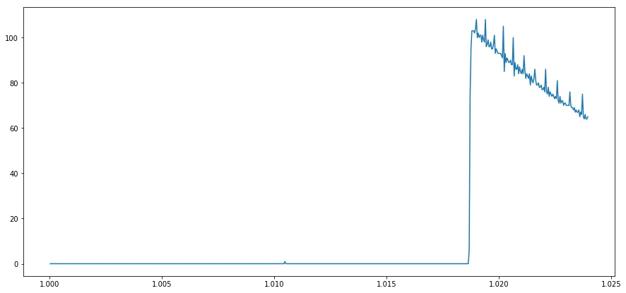
3.2. NXCALS
In the next step we query NXCALS for BLM running sum 1.
- Signal Query of Loss Running Sum 1
In [17]:
loss_rs01_df = QueryBuilder().with_nxcals(spark) \
    .with_duration(t_start=start_time_date, duration=[(100, 's'), (200, 's')]) \
    .with_query_parameters(nxcals_system='CMW', signal='%s:LOSS_RS01'%blm_names_df.at[0, 'blmNames']) \
    .signal_query() \
    .convert_index_to_sec() \
    .synchronize_time() \
    .dfs[0]

loss_rs01_df.plot()
Out[17]:
<matplotlib.axes._subplots.AxesSubplot at 0x7fb5eea90c18>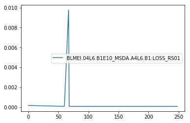
4. Feature Query All BLMs for a Single Crate
Due to the large number of BLMs, the query and plotting of them is impractical in this environment. In fact there are dedicated applications for this purpose. In the following, we will demonstrate the feature engineering (mean, std, min, max value) for the BLM signals stored in PM and NXCALS.
In [18]:
features = ['mean', 'std', 'max', 'min']
4.1. Post Mortem
PM does not support calculation of features on the database (which is profitable from the communication and computation time perspective). Therefore, we need to query the raw signals and afterwards perform feature engineering.
- pmLogHistory1310msThresholds
In [19]:
blm_thresholds_features_row_df = FeatureBuilder().with_multicolumn_signal(blm_thresholds_df) \
    .calculate_features(features=features, prefix='threshold') \
    .convert_into_row(index=lhc_context_df.index) \
    .dfs
- pmTurnLoss
In [20]:
blm_turn_loss_features_row_df = FeatureBuilder().with_multicolumn_signal(blm_turn_loss_df) \
    .calculate_features(features=features, prefix='turn_loss') \
    .convert_into_row(index=lhc_context_df.index) \
    .dfs
4.2. NXCALS
NXCALS ecosystem brings the cluster computing capabilities to the logging databases. It allows developing analysis code witht the Spark API. The pyeDSL encapsulates Spark API and provides a coherent feature engineering query. In other words, features are calculated on the cluster where the data is stored unlike the PM for which the calculation is performed locally. The table of BLM signal names was prepared by Christoph Wiesener.
- Get signal names from MappingMetadata
In [21]:
blm_nxcals_df = MappingMetadata.get_blm_table()
blm_nxcals_df['LOSS_RS01'] = blm_nxcals_df['Variable Name'].apply(lambda x: '%s:LOSS_RS01' % x)
blm_nxcals_df['LOSS_RS09'] = blm_nxcals_df['Variable Name'].apply(lambda x: '%s:LOSS_RS09' % x)
blm_nxcals_df.head()
Out[21]:
| Subscription Id | Device Name | PPM | Cycle Bound | Class Name | Accelerator | Property Name | Selector | Enabled | Timestamp Type | … | UF: Fixed rate | UF: Rounding type | UF: Rounding compare | Responsible | Status Time | Last Check Time | Status | Error Message | LOSS_RS01 | LOSS_RS09 | |
|---|---|---|---|---|---|---|---|---|---|---|---|---|---|---|---|---|---|---|---|---|---|
| 0 | 143020 | BLMMI.31L2.B2I14_V | False | False | BLM_MONITOR_V | LHC | Acquisition | NaN | True | ACQUISITION | … | NaN | NaN | NaN | Kamil Henryk Krol | 2019-03-01T08:43:40.662+0000 | 2020-04-14T09:46:57.011+0000 | VALIDATION_IN_ERROR | Failed to connect to server 'LHC_CONCENTRATION… | BLMMI.31L2.B2I14:LOSS_RS01 | BLMMI.31L2.B2I14:LOSS_RS09 |
| 1 | 143002 | BLMDI.9822.B2L10_13.200_DUMP_V | False | False | BLM_MONITOR_V | LHC | Acquisition | NaN | True | ACQUISITION | … | NaN | NaN | NaN | Kamil Henryk Krol | 2019-10-23T04:30:47.616+0000 | 2020-04-14T09:46:56.964+0000 | VALIDATION_IN_ERROR | Failed to connect to server 'LHC_CONCENTRATION… | BLMDI.9822.B2L10_13.200_DUMP:LOSS_RS01 | BLMDI.9822.B2L10_13.200_DUMP:LOSS_RS09 |
| 2 | 142984 | BLMDI.9724.B1R10_2.450_DUMP_V | False | False | BLM_MONITOR_V | LHC | Acquisition | NaN | True | ACQUISITION | … | NaN | NaN | NaN | Kamil Henryk Krol | 2019-10-23T04:30:47.758+0000 | 2020-04-14T09:46:56.771+0000 | VALIDATION_IN_ERROR | Failed to connect to server 'LHC_CONCENTRATION… | BLMDI.9724.B1R10_2.450_DUMP:LOSS_RS01 | BLMDI.9724.B1R10_2.450_DUMP:LOSS_RS09 |
| 3 | 143024 | BLMTI.05L1.B2E10_TCLVW.5L1.B2_V | False | False | BLM_MONITOR_V | LHC | Acquisition | NaN | True | ACQUISITION | … | NaN | NaN | NaN | Kamil Henryk Krol | 2019-03-29T14:16:44.600+0000 | 2020-04-14T09:46:57.020+0000 | VALIDATION_IN_ERROR | Failed to connect to server 'LHC_CONCENTRATION… | BLMTI.05L1.B2E10_TCLVW.5L1.B2:LOSS_RS01 | BLMTI.05L1.B2E10_TCLVW.5L1.B2:LOSS_RS09 |
| 4 | 143022 | BLMMI.31L2.B2I15_V | False | False | BLM_MONITOR_V | LHC | Acquisition | NaN | True | ACQUISITION | … | NaN | NaN | NaN | Kamil Henryk Krol | 2019-03-01T08:43:40.657+0000 | 2020-04-14T09:46:57.022+0000 | VALIDATION_IN_ERROR | Failed to connect to server 'LHC_CONCENTRATION… | BLMMI.31L2.B2I15:LOSS_RS01 | BLMMI.31L2.B2I15:LOSS_RS09 |
5 rows × 25 columns
- Run a feature query with pyeDSL: Running Sum 1
In [22]:
loss_rs01_features_row_df = QueryBuilder().with_nxcals(spark) \
    .with_duration(t_start=start_time_date, duration=[(100, 's'), (200, 's')]) \
    .with_query_parameters(nxcals_system='CMW', signal=list(blm_nxcals_df['LOSS_RS01'])) \
    .feature_query(features=features) \
    .convert_into_row(lhc_context_df.index) \
    .df

loss_rs01_features_row_df
Out[22]:
| BLMTI.04L6.B2I10_TCSP.A4L6.B2:LOSS_RS01_std | BLMTI.04L6.B2I10_TCSP.A4L6.B2:LOSS_RS01_max | BLMTI.04L6.B2I10_TCSP.A4L6.B2:LOSS_RS01_min | BLMTI.04L6.B2I10_TCSP.A4L6.B2:LOSS_RS01_mean | BLMQI.07R4.B2E20_MQM:LOSS_RS01_std | BLMQI.07R4.B2E20_MQM:LOSS_RS01_max | BLMQI.07R4.B2E20_MQM:LOSS_RS01_min | BLMQI.07R4.B2E20_MQM:LOSS_RS01_mean | BLMBI.31R6.B0T10_MBB-MBA_30R6:LOSS_RS01_std | BLMBI.31R6.B0T10_MBB-MBA_30R6:LOSS_RS01_max | … | BLMQI.30R3.B2E10_MQ:LOSS_RS01_min | BLMQI.30R3.B2E10_MQ:LOSS_RS01_mean | BLMQI.23L6.B2I30_MQ:LOSS_RS01_std | BLMQI.23L6.B2I30_MQ:LOSS_RS01_max | BLMQI.23L6.B2I30_MQ:LOSS_RS01_min | BLMQI.23L6.B2I30_MQ:LOSS_RS01_mean | BLMQI.28L4.B2E30_MQ:LOSS_RS01_std | BLMQI.28L4.B2E30_MQ:LOSS_RS01_max | BLMQI.28L4.B2E30_MQ:LOSS_RS01_min | BLMQI.28L4.B2E30_MQ:LOSS_RS01_mean | |
|---|---|---|---|---|---|---|---|---|---|---|---|---|---|---|---|---|---|---|---|---|---|
| 4647 | 6.278608 | 16.611908 | 0.0 | 2.373363 | 0.0 | 0.000091 | 0.000091 | 0.000091 | 0.000081 | 0.000272 | … | 0.000091 | 0.000091 | 0.0 | 0.000091 | 0.000091 | 0.000091 | 0.0 | 0.000091 | 0.000091 | 0.000091 |
1 rows × 15628 columns
- Run a feature query with pyeDSL: Running Sum 9
In [23]:
loss_rs09_features_row_df = QueryBuilder().with_nxcals(spark) \
    .with_duration(t_start=start_time_date, duration=[(100, 's'), (200, 's')]) \
    .with_query_parameters(nxcals_system='CMW', signal=list(blm_nxcals_df['LOSS_RS09'])) \
    .feature_query(features=features) \
    .convert_into_row(lhc_context_df.index) \
    .df

loss_rs09_features_row_df
Out[23]:
| BLMEL.06R8.B2E30_MSIA:LOSS_RS09_std | BLMEL.06R8.B2E30_MSIA:LOSS_RS09_max | BLMEL.06R8.B2E30_MSIA:LOSS_RS09_min | BLMEL.06R8.B2E30_MSIA:LOSS_RS09_mean | BLMTI.04R3.B1I10_TCSG.4R3.B1:LOSS_RS09_std | BLMTI.04R3.B1I10_TCSG.4R3.B1:LOSS_RS09_max | BLMTI.04R3.B1I10_TCSG.4R3.B1:LOSS_RS09_min | BLMTI.04R3.B1I10_TCSG.4R3.B1:LOSS_RS09_mean | BLMBI.23L8.B0T10_MBA-MBB_22L8:LOSS_RS09_std | BLMBI.23L8.B0T10_MBA-MBB_22L8:LOSS_RS09_max | … | BLMQI.19R8.B1I10_MQ:LOSS_RS09_min | BLMQI.19R8.B1I10_MQ:LOSS_RS09_mean | BLMES.04R6.B2I10_MSDB.A4R6.B2:LOSS_RS09_std | BLMES.04R6.B2I10_MSDB.A4R6.B2:LOSS_RS09_max | BLMES.04R6.B2I10_MSDB.A4R6.B2:LOSS_RS09_min | BLMES.04R6.B2I10_MSDB.A4R6.B2:LOSS_RS09_mean | BLMTS.04R1.B1E10_TANAR.4R1:LOSS_RS09_std | BLMTS.04R1.B1E10_TANAR.4R1:LOSS_RS09_max | BLMTS.04R1.B1E10_TANAR.4R1:LOSS_RS09_min | BLMTS.04R1.B1E10_TANAR.4R1:LOSS_RS09_mean | |
|---|---|---|---|---|---|---|---|---|---|---|---|---|---|---|---|---|---|---|---|---|---|
| 4647 | 0.000002 | 0.00002 | 0.000011 | 0.000016 | 0.000016 | 0.000114 | 4.502000e-07 | 0.000069 | 1.453712e-08 | 2.292000e-07 | … | 1.657000e-07 | 1.828400e-07 | 0.000484 | 0.02625 | 0.02509 | 0.025558 | 0.001239 | 0.02258 | 0.01969 | 0.02131 |
1 rows × 15628 columns
5. Final Row
Eventually, we put together all rows into a single one that can be stored in the persistent storage. The code of this notebook can be extracted into a job collecting historical data representing BLM signals during the operation of the LHC.
In [24]:
pd.concat([lhc_context_df, blm_thresholds_features_row_df, blm_turn_loss_features_row_df, loss_rs01_features_row_df, loss_rs09_features_row_df], axis=1)
Out[24]:
| OVERALL_ENERGY | OVERALL_INTENSITY_1 | OVERALL_INTENSITY_2 | BEAM_MODE | timestamp_blm | aGXpocTotalIntensityB1 | aGXpocTotalMaxIntensityB1 | aGXpocTotalIntensityB2 | aGXpocTotalMaxIntensityB2 | timestamp_abort_gap | … | BLMQI.19R8.B1I10_MQ:LOSS_RS09_min | BLMQI.19R8.B1I10_MQ:LOSS_RS09_mean | BLMES.04R6.B2I10_MSDB.A4R6.B2:LOSS_RS09_std | BLMES.04R6.B2I10_MSDB.A4R6.B2:LOSS_RS09_max | BLMES.04R6.B2I10_MSDB.A4R6.B2:LOSS_RS09_min | BLMES.04R6.B2I10_MSDB.A4R6.B2:LOSS_RS09_mean | BLMTS.04R1.B1E10_TANAR.4R1:LOSS_RS09_std | BLMTS.04R1.B1E10_TANAR.4R1:LOSS_RS09_max | BLMTS.04R1.B1E10_TANAR.4R1:LOSS_RS09_min | BLMTS.04R1.B1E10_TANAR.4R1:LOSS_RS09_mean | |
|---|---|---|---|---|---|---|---|---|---|---|---|---|---|---|---|---|---|---|---|---|---|
| 4647 | 25098.0 | 16537 | 17110 | STABLE | 1448260133517488525 | 2.457193e+10 | 8.560893e+08 | 4.608540e+09 | 1.917766e+08 | 1448260134624467000 | … | 1.657000e-07 | 1.828400e-07 | 0.000484 | 0.02625 | 0.02509 | 0.025558 | 0.001239 | 0.02258 | 0.01969 | 0.02131 |
1 rows × 33314 columns