The development of the API has been driven by the need of providing a general-purpose framework for cre- ating signal monitoring applications (signal query, processing, along with visualization and storage of results) and a dedicated workflow. Initially, the focus was put on migrating existing applications that may become incompatible with the introduction of the NXCALS ecosystem (busbar and magnet resistance monitoring) or could be enhanced by the use of machine learning techniques (quench heater discharge analysis). We follow a four-step process in developing monitoring applications as shown.

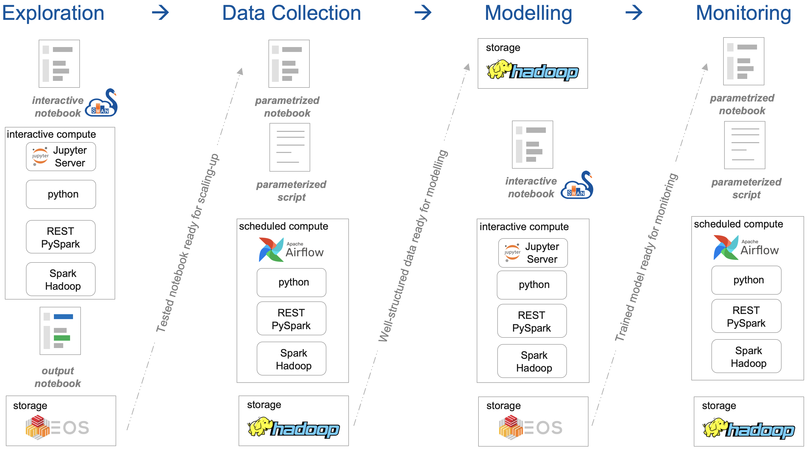
An equally important aspect of developing monitoring application has been the development of a monitoring pipeline matching the present computing infrastructure provided by the IT department. The definition of a signal monitoring workflow included selection of a scheduling system, persistent database for storage, and visualization techniques for displaying the results.

1. Exploration

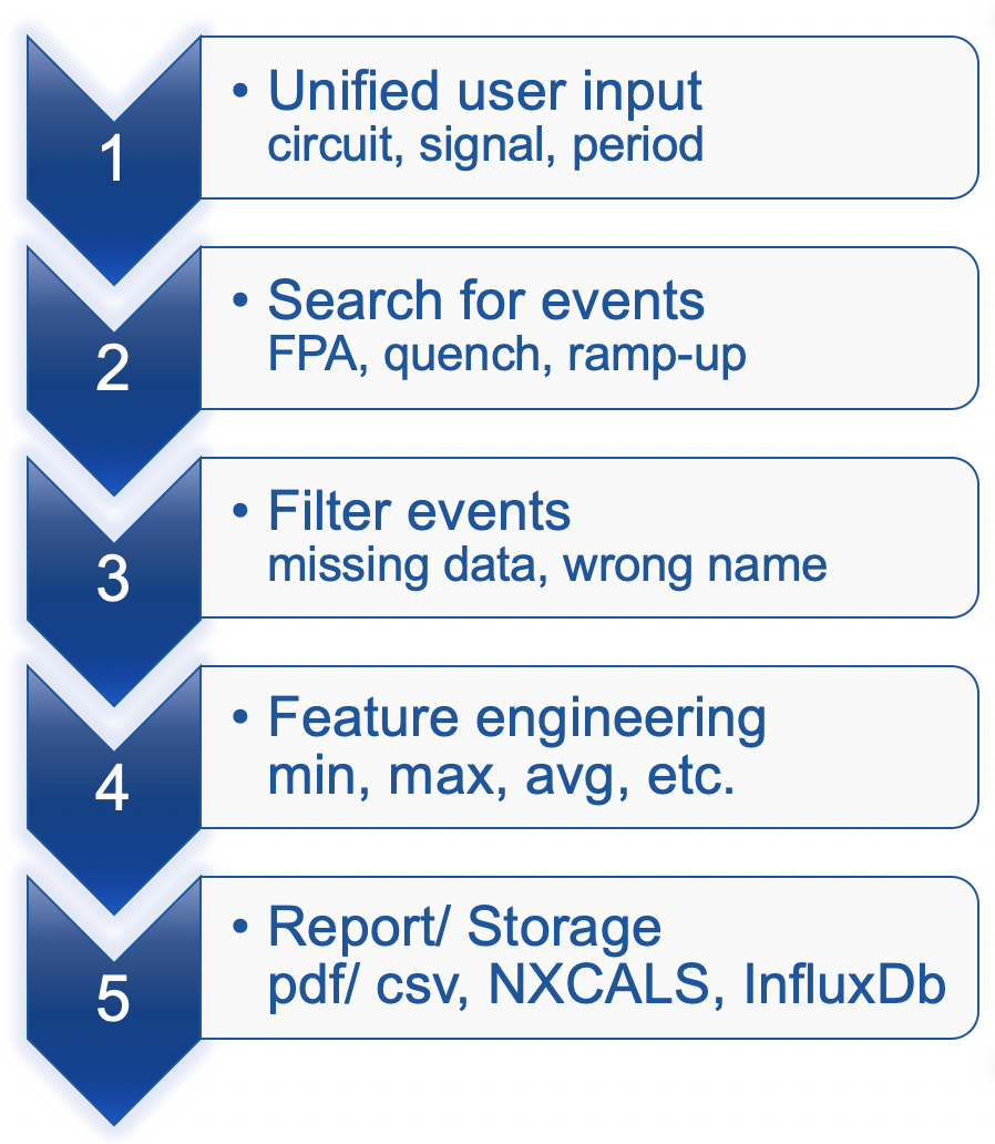
The Exploration step aims at getting the features right, i.e., prototyping a monitoring application for a sin- gle event. This process starts with gathering the functional specification from system experts, which can be characterized by five stages.

Naturally, this is an arbitrary division of the development process. Nonetheless we found it helpful in prototyping the monitoring applications.

1.1. Unified User Input

The first part of creating an acquisition application is to select relevant circuits and signals from the Metadata sub-package. Then, a period of time with a considered event should be specified (e.g., a current ramp-up, an FPA, a magnet quench).

1.2. Search for Events

Once the user input is specified, we query databases in order to find the considered event. This typically involves either querying the NXCALS database for the beam mode/power converter current or the PM database for FGC and/or QPS events.

1.3. Filter Events

After finding relevant events and/or periods of time they are validated. This includes cross-checking the beam mode against the power converter current or name of a source for an event obtained from the PM database.

1.4. Feature Engineering

The core of the acquisition step is the extraction of characteristic features representing a signal. For that pur- pose we use both the raw signals (in order to check whether a threshold was reached) and processed ones. The processing involves taking averages, derivatives, standard deviations and applying different types of filtering for the sake of numerical stability.

We developed methods for extracting simple features (min, max, mean, std, median, sum, etc.) as well as more elaborate ones (resistance, time constant, frequency spectrum, etc.). Furthermore, depending on the use case, we extract trends (e.g., change of the average value over time) and correlations (to signals in the same or a circuit with similar topology and/or its value from the past).

1.5. Report/Storage

Finally, the results of the acquisition step are summarised as a report (by exporting a notebook). After vali- dation and testing, the result of this step is a single row with features characterising the analyzed event saved to the persistent storage. In addition, the row is enriched with some context information (beam mode, energy, fill number, etc.). This concludes the acquisition step and opens a way for gathering the historical data in the exploration step.

2. Data Collection

The goal of the Data Collection step is to get the right features at scale. To this end, we compact a notebook created in the acquisition step and embed in the API. Then, the dedicated methods are executed over an extended period of time in order to create a table with rows corresponding to events (e.g., machine cycles, FPAs, quenches) and columns corresponding to features representing analyzed signals.

Since SWAN is not suited for executing long-running data-gathering application, this step required a dedi- cated solution for controlling the execution (eventually achieved with the Apache Airflow).

3. Modelling

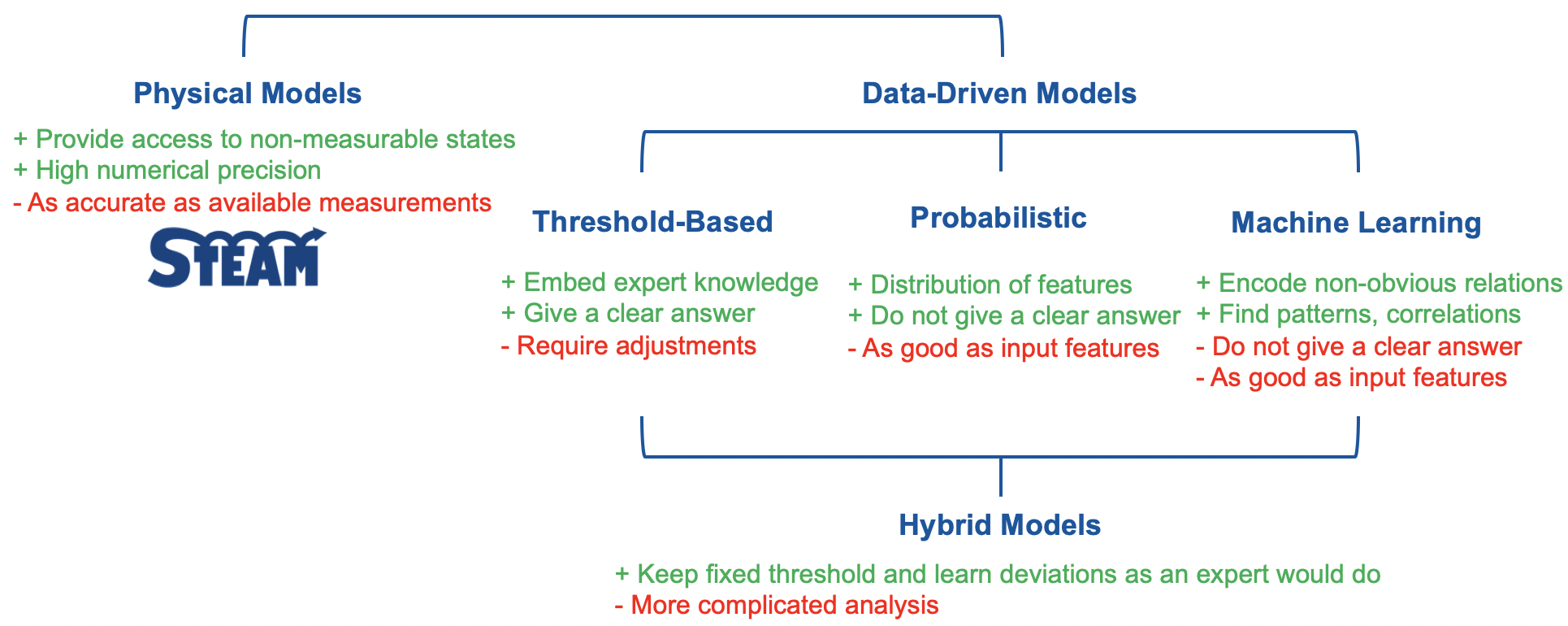
Once a historical data is gathered, a system modelling is carried out. There is a large variety of modelling meth- ods available to encode the historical data in a compact form, which then can be used for signal monitoring. One grouping of methods divides models into: (i) physical; (ii) and data-driven. The physical models rely on equations describing the physics in order to represent historical data. The data-driven models use historical data and general-purpose equations to encode the system behaviour. The data-driven models are subdivided further into threshold-based models, probabilistic models and machine learning-based models. Figure below presents different types of models foreseen for performing on-line monitoring of LHC superconducting circuits along with their advantages and disadvantages.

For the data-driven models, the left-to-right order can be interpreted in several ways:

• from a clear yes/no answer to vague probabilistic distributions;
• from zero predictive power to a certain predictive potential;
• from fully deterministic algorithms and clear answer, to deterministic algorithms and probabilistic answer, to non-deterministic algorithms and probabilistic answer;
• from low, to moderate, to high computational cost in order to develop and train the model;
• from full trust to result, to high-degree of trust, to low-level of trust;

3.1. Physical Models

The physical models typically rely on a set of ordinary differential-algebraic equations (e.g., network model of a circuit or a magnet) or partial differential-algebraic equations (e.g., a Finite-Element Model of a magnet or a diode). This type of modelling requires a deep understanding of the underlying physics. In order to use a physical model, one needs to perform its verification (to check if the equations are solved correctly) and validation (to check if the correct equations are solved). The verification is carried out be comparing a model to existing, trusted models or analytical solutions to a given problem. The validation involves comparison of signals obtained with a model to available measurements. Thus, a model is as good as the measurements and is always wrong, i.e., a physical model by its very nature is not capable of reproducing the reality. However, a validated physical model can provide access to non-measurable variables (e.g., internal distribution of the temperature in a magnet) at a very fine temporal resolution (e.g., voltage feelers in RB and RQ circuits have rather low sampling rate capturing the dominant behavior). In addition, physical models are helpful in case a circuit does not exist (either undergoes a considerable case as in the case of the modified RB circuit or is still to be assembled as for the inner triplet circuit). In this case, a model is useful for providing reference signals for monitoring applications.

3.2. Threshold-Based Models

In threshold-based models, the measured value of a feature is compared to a fixed threshold giving a clear ok/not ok answer. There is no requirement on the size of a dataset needed to define the thresholds. In fact, one can based the thresholds on the design specification, numerical models, etc. In case, there is a historical data available, one can set the threshold as an average values with a certain safety factor. With the ageing of a system, the thresholds may require adjustment limiting the use of this method for monitoring.

3.3. Probabilistic Models

The probabilistic models fit probability density functions (e.g., Gaussian, binomial, Poisson, etc.) from theavailable historical data. A model constructed this way can be used in monitoring applications to provide aninformation on the confidence intervals. In this case, the larger a dataset, the better (following the Law ofLarge Numbers). This method allows accounting for a natural distribution of calculated features across thehistorical data and/or the population of similar systems. A probabilistic model provides the confidence interval up to a finite accuracy (never reaching 1).

3.4. Machine Learning Models

Machine learning is a term representing a class of algorithms in which there is a very limited to no informationabout the modelled behavior. An example of a machine learning algorithm is linear regression which finds coefficients of a linear function from the input data (a more interesting case is a multi-dimensional linear regression giving rise to support vector machines). Traditionally, the machine learning algorithms are grouped into

• supervised - in this case, the dataset contains labels indicating to what category an input vector belongs.A model is trained to achieve a high rate of accuracy in mapping the input vector to its label so that itcan be used for prediction, i.e., proposing a label for an unseen input vector. This class of algorithms includes classification methods for categorical data, and regression methods for continuous data. Common classification methods include: k-nearest neighbours, neural networks, support vector machines. Some of the popular regression methods are: (non)-linear regression, neural networks.
• unsupervised - for datasets without labelled information. A goal of the model is to recognize clusters ofinput vectors that can be further labelled by a user. Among suitable algorithms, there are hidden Markov models, k-means (mediods) models, gaussian-mixture models.
•  semi-supervised - is a mixture of above mentioned models in which only some input vector are labeledand/or labelling progresses with the use of the models, i.e., the unsupervised methods reveal hiddenpatterns in data, which are then labelled and used as an input to the supervised methods.Since the output of a model relies heavily on the input dataset, one should follow a three-step process(testing, training, and validation) to avoid under/over fitting of the input data.

3.5. Hybrid Models

An interesting approach is a combination of aforementioned models. A proof-of-concept has been demonstrated for the case of monitoring quench heater discharges in which a threshold-based model was combined with a support vector machine. During observation the threshold have been adjusted in order to ensure that good discharges are properly classified. In this setup, the threshold-based method operates with fixed threshold, while the support vector machine was mimicking the expert-learning process to adjust the thresholds in order to properly classify a discharge.

4. Monitoring

Little number of faults makes it difficult to encode a faulty pattern of a signal leading to an anomaly. Thus, we undertake another approach inspired by methodology proposed by the Predictail company. This methodology uses both historical and on-line data to classify whether a feature is expected or indicates an anomaly.

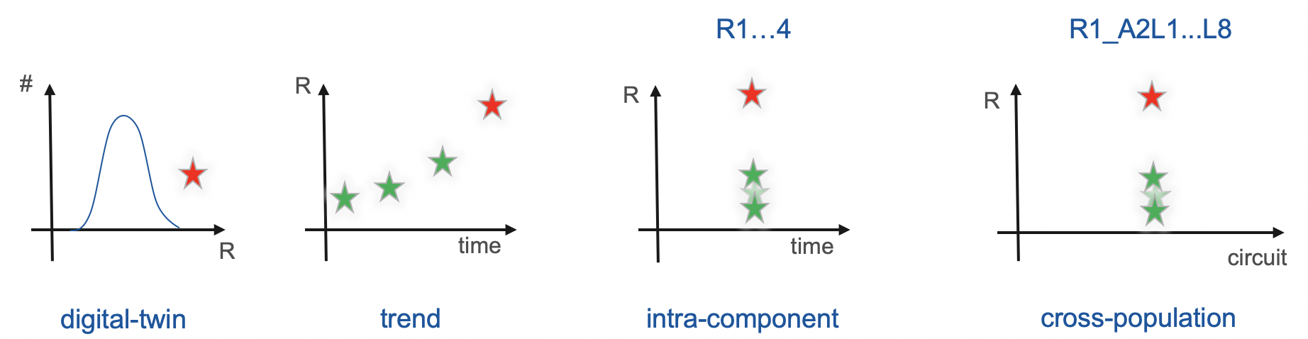
We envision to use the following methods based on historical data:

1. digital-twin - to compare value predicated by a model (any of the aforementioned models) for a given operational point of the on-line data to the measured feature. If the measured feature differs from the one predicted by a model, a warning should be raised.
2. trend - based on the average value of a feature observed in historical data, we derive trends. Assuming a certain extrapolation function, we can conclude, when the average value could reach a safety threshold informing about a need for intervention.

For the online data, we plan to use the following methods:

1. intra-component - compares signal and/or its feature across redundant copies of a system in the same circuit (e.g., quench heater discharge profiles)

2. cross-population - compares signal and/or its feature across instances of a system in circuits with the same/similar topology.